Expanding the Quality–Coverage Frontier with Competitive Flow Matching

Wenxuan Peng^1,2Richard Zhang²Haitian Zheng²Jaskirat Singh²Tsai-Shien Chen²Eli Shechtman²Bharath Hariharan¹Hadar Averbuch-Elor¹Zongze Wu²

¹Cornell University²

arXiv

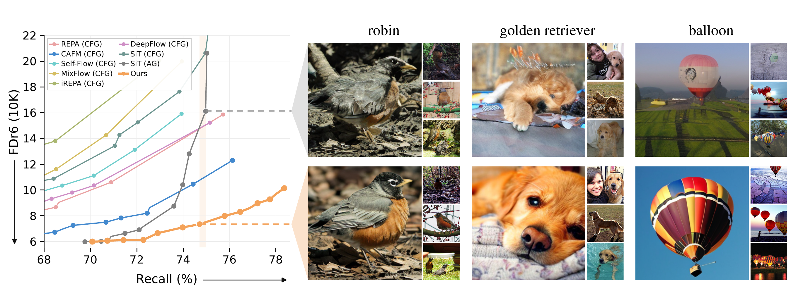
A successful generative model has two essential aspects: (1) high-fidelity, where each randomly drawn sample looks realistic, and (2) broad coverage, where the full data distribution is well-represented. Inference-time techniques such as classifier-free guidance raise quality, but at the cost of coverage. In this work, we demonstrate improvements in both quality and coverage, pushing the frontier significantly.

Figure 1. Left: ImageNet-256 quality–coverage frontiers, with Competitive Flow Matching shown in orange. Right: paired robin, golden retriever and balloon samples before (top) and after (bottom) applying our approach to SiT. — The plot on the left shows that while progress has indeed been made in **quality** (moving down the y-axis), the **coverage** of the distribution (x-axis) has been underexplored. Our method reaches substantially stronger performance in the **high-coverage regime**.

This is illustrated on the right using random samples, comparing samples obtained using the same class condition and initial noise before (top) and after (bottom) applying our approach over the SiT baseline.

ImageNet-256. Curves are obtained by sweeping each method’s inference-time guidance. CFG and AG denote classifier-free guidance and AutoGuidance, respectively.

TL;DR: Better image quality, with broader coverage.

We post-train flow matching generators by letting multiple predictions compete to explain each training target. With less than 3% of the original pretraining compute, this substantially expands the quality–coverage frontier shown above, with the largest gains at broad coverage.

Intuition: Same noisy state, multiple answers

Improving generation quality while maintaining broad coverage remains challenging. We hypothesize this limitation stems from a basic property of the flow matching objective.

We revisit flow matching through a 1D toy example: transporting a unimodal source distribution to an imbalanced bimodal target distribution.

Pair APair BFM prediction

This motivates our key insight: accommodate multiple alternatives with multiple predictions.

Method: What if the model could make `K` guesses?

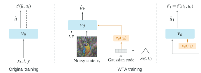
Instead of asking a single prediction to fit multiple possible targets, we give the model more room. We allow the model to make K guesses for the same noisy state and use only the best-matching guess to fit the current training target.

Auxiliary conditioning architecture. A low-dimensional Gaussian code z is mapped through c phi to condition the same velocity predictor v theta, alongside the noisy state, time and class condition.

To allow the model to make multiple predictions for the same noisy state, we introduce a low-dimensional Gaussian code z as auxiliary conditioning.

Different samples of z allow the same model to produce different velocity predictions.

Winner-take-all training

During training, we sample K auxiliary codes, yielding K candidate velocity predictions for the same intermediate state. Only the best-matching candidate receives the regression loss—a winner-take-all (WTA) objective.

Standard Flow Matching makes one prediction and fits it to the sampled target. WTA evaluates K predictions from the same shared model using different auxiliary codes, compares each with the same target, and backpropagates only through the minimum-loss candidate, highlighted in green.

We now return to the 1D toy example to see what competitive training changes.

Different codes, different predictions

The same auxiliary-conditioned predictor, with lambda multiplying the conditioning signal c phi of z k. — FM prediction

After WTA training

Code 1Code 2

After WTA training, different auxiliary codes allow the model to produce different velocity predictions for the same noisy state. In this toy example, the predictions point toward the two target modes.

Image generation: Better quality, broader coverage

A stronger generator after just 10 epochs of post-training.

Competitive post-training improves generation quality, including at matched and higher coverage than pretrained SiT. The same model also gains its own control: varying λ moves it from high-precision to broader-coverage generation.

Better quality across the displayed range. The orange points lie below pretrained SiT, with some also reaching further to the right.

Our model turns guidance into a win-win at high coverage.

Competitive post-training changes how the model responds to inference-time guidance. For pretrained SiT, stronger guidance improves quality at the cost of coverage. At high-coverage settings, our model instead improves quality while preserving—and sometimes increasing—Recall.

Follow the paths downward. Our high-coverage settings gain quality while retaining coverage. The bold orange line shows the resulting frontier.

Guided comparison under the standard 50K-sample evaluation
Method	(a) Performance @ best FD_r,6 (50K)										(b) Performance @ Recall ≈ 67% (50K)
	Multi-encoder Fréchet distances ↓						FD_r,6 ↓	Recall (%) ↑	Precision (%) ↑	IS ↑	Multi-encoder Fréchet distances ↓						FD_r,6 ↓	Recall (%) ↑	Precision (%) ↑	IS ↑
	FID (ADM)	ConvNeXt	DINOv2	MAE	SigLIP	CLIP	FD_r,6 ↓	Recall (%) ↑	Precision (%) ↑	IS ↑	FID (ADM)	ConvNeXt	DINOv2	MAE	SigLIP	CLIP	FD_r,6 ↓	Recall (%) ↑	Precision (%) ↑	IS ↑
CAFM	3.30	85.58	51.49	0.13	5.06	58.31	4.86	57.1	83.8	342.7	3.84	225.73	135.82	0.24	10.91	106.67	9.84	67.3	72.1	181.9
REPA	4.79	132.70	52.50	0.19	5.69	60.93	5.65	49.7	88.0	388.8	6.42	302.84	171.30	0.37	14.43	136.53	13.13	67.2	69.7	162.5
MixFlow^†	6.52	156.09	65.02	0.20	6.40	67.52	6.49	46.9	88.6	396.1	9.35	495.73	252.08	0.50	21.91	169.85	18.57	66.0 (below 67%)	68.0	133.5
Self-Flow^†	6.37	147.99	55.50	0.18	6.05	60.74	5.94	46.5	89.8	388.1	7.63	400.46	197.52	0.35	16.29	143.51	14.51	66.1 (below 67%)	69.4	138.1
StableVM	5.47	140.84	52.32	0.18	5.75	60.29	5.72	48.0	88.6	391.1	7.45	360.07	188.04	0.38	15.46	142.35	14.14	67.9	68.7	147.3
DeepFlow	5.64	143.20	52.50	0.19	5.84	60.50	5.83	48.2	88.8	398.6	7.16	359.93	186.26	0.38	15.47	139.92	14.00	67.3	68.7	148.2
iREPA^†	7.26	170.67	73.12	0.28	9.50	71.03	7.99	40.5	90.8	373.4	9.81	551.60	256.33	0.49	22.97	160.22	18.81	65.2 (below 67%)	67.9	117.6
SiT (CFG)^†	6.52	150.02	62.21	0.20	6.53	64.86	6.40	46.6	89.2	383.7	11.17	572.67	275.86	0.47	21.39	177.22	19.22	66.9 (below 67%)	66.3	118.6
SiT (AG)^†	2.13	85.92	50.46	0.11	5.26	52.29	4.53	62.2	78.1	236.9	11.17	572.67	275.86	0.47	21.39	177.22	19.22	66.9 (below 67%)	66.3	118.6
Ours	2.29	77.44	46.13	0.13	5.24	49.06	4.44	60.4	79.9	258.2	2.20	122.93	69.43	0.20	6.72	61.19	5.91	67.4	73.0	210.5

The advantage grows at broader coverage.

Lowest FD_r,6 in both settings, with a larger advantage at high coverage.

ImageNet-256 · 50-step Euler sampling · FD_r,6 averages six normalized component distances (lower = better overall generation quality); higher Recall = broader coverage · Guidance uses AutoGuidance.

† marks methods whose highest measured Recall is below 67%; these Recall values are gray in (b).

Generalizing to an even stronger generator.

We also post-train the already strong RAEv2 generator with our method, expanding its quality–coverage frontier in just 10 epochs.

RAEv2 performance comparison, 50K samples
Method	Performance @ best FD_r,6 (50K)				Performance @ Recall ≈ 70% (50K)
Method	FD_r,6 ↓	Recall (%) ↑	Precision (%) ↑	IS ↑	FD_r,6 ↓	Recall (%) ↑	Precision (%) ↑	IS ↑
RAEv2	2.07	64.72	79.39	261.68	16.83	69.09	52.39	111.47
Ours	2.02	65.71	78.30	265.82	3.18	70.32	71.25	182.39

Analysis: What does competition change?

Competitive post-training improves the base model itself. With auxiliary conditioning removed (λ = 0), the model shifts toward higher Precision and lower Recall than its pretrained counterpart. We vary K—the number of competing predictions during training—to examine the role of competition in SiT.

More competition, a higher-fidelity base model.

At 50 sampling steps, increasing K from 1 to 32 raises Precision and lowers FDr6. Dashed lines show pretrained SiT; K=1 stays close to these references. — With `K` = 1, post-training leaves SiT nearly unchanged. As more predictions compete, Precision rises and FD_r,6 falls under 50-step sampling.

The effect is stronger with fewer sampling steps.

Precision and FDr6 for 4-, 8-, and 50-step sampling as K increases from 1 to 256. The few-step quality gap narrows with stronger competition. — As `K` increases, 4- and 8-step generation improve substantially, narrowing the gap to 50-step generation. Increasing `K` adds computation during training, without increasing sampling cost—shifting compute from inference to training.

Cite

BibTeX

@misc{peng2026cfm,
  title  = {Expanding the Quality--Coverage Frontier with Competitive Flow Matching},
  author = {Peng, Wenxuan and Zhang, Richard and Zheng, Haitian and
            Singh, Jaskirat and Chen, Tsai-Shien and Shechtman, Eli and
            Hariharan, Bharath and Averbuch-Elor, Hadar and Wu, Zongze},
  year   = {2026}
}

Expanding the Quality–Coverage Frontier with Competitive Flow Matching

Intuition: Same noisy state, multiple answers